Probability Distribution 1#

A probability distribution is a list of all of the possible outcomes of a random variable along with their corresponding probability values.

Random Variable#

A random variable is any variable whose outcome is a random event. It can be discrete (e.g., outcome of a coin toss or the roll of a die) as well as continuous (e.g., the heights of students in the class or the time needed by athletes to complete a 100 m race).

from scipy.stats import binom
from scipy.stats import norm
import numpy as np 
import matplotlib.pyplot as plt
import seaborn as sns
np.random.seed(10)

plt.style.use('seaborn')

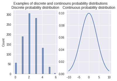
fig, axes = plt.subplots(1, 2)
fig.suptitle('Examples of discrete and continouns probability distributions')

data = binom.rvs(n=6, p=0.4, size=1000)
sns.histplot(data, ax=axes[0]);
axes[0].set_title('Discrete probability distribution')

x = np.linspace(-10, 10, 200)
y = norm.pdf(x, 0, 4)
sns.lineplot(x=x, y=y, ax=axes[1]);
axes[1].set_title('Continuous probability distribution');

../../_images/Probability Distribution 1_2_0.png

Discrete Random Variables#

When a probability function is used to describe a discrete random variable (denoted by \(X\)), we call this function as probability mass function (PMF). Formally, a PMF is written as:

\[ \begin{equation} f(x) = p(X=x) \end{equation} \]

\(p(x)\) is called as a probability mass function if it satisfies the following conditions:

\(p(x) > 0\)
\(p(x) <= 1\)
\(\sum_{x} p(x) = 1\)

In the example of an unbiased dice roll, the probability of landing the number 2 (denoted by \(x\)) is represented as \(p(X=x) = \frac{1}{6}\). The PMF just returns the probability of the outcome at a given point \(x\).

Continuous Random Variables#

When a probability function is used to describe a continuous random variable (denoted by \(X\)), we call this function as probability distribution function (PDF). It is meaningless to represent a probability with any discrete value. To get the probability from a probability density function we need to find the area under the curve. We can then find the probability that the ourcome lies within an interval by calculating the area under the curve. Formally, an interval is used to represent the probability within that interval \(X \in (x, x + \delta x)\). \(p(x)\delta x\) is the probability that \(X \in (x, x+\delta x)\) as \(\delta x \rightarrow 0\). The probability density function satisfies the following criteria:

\(p(x) \ge 0\)
\(\int_{-\infty}^{+\infty}p(x)dx = 1\)
\(\int_a^b p(x)dx = P(a \lt X \lt b)\)

from scipy import stats

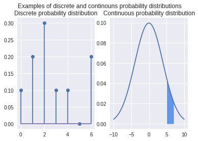
fig, axes = plt.subplots(1, 2)
fig.suptitle('Examples of discrete and continouns probability distributions')

xk = np.arange(0, 7)
pk = (0.1, 0.2, 0.3, 0.1, 0.1, 0.0, 0.2)
custm = stats.rv_discrete(name='custm', values=(xk, pk))
data = custm.pmf(xk)
plt.subplot(1, 2, 1)
plt.title('Discrete probability distribution')
plt.stem(data)

x = np.linspace(-10, 10, 200)
y = norm.pdf(x, 0, 4)
sns.lineplot(x=x, y=y, ax=axes[1]);
axes[1].fill_between(x[150:170], y[150:170], color='cornflowerblue')
axes[1].set_title('Continuous probability distribution');

../../_images/Probability Distribution 1_5_0.png

Notation#

\(p(.)\) can mean different things depending on the context.
1. \(p(X)\) denotes the distribution (PMF/PDF) of a random variable \(X\).
2. \(p(X=x)\) or \(p(x)\) denotes the proability or probability density at point \(x\). The actual meaning needs to be understood from context.
The following means drawing from a random sample from the distribution \(p(X)\):

\[ \begin{equation} x \sim p(X) \end{equation} \]

Joint Distributions#

Often in real life, we are interested in multiple random variables that are related to each other. For example, let us choose a random set of students in a classroom. We would like to study the number of students in the classroom, their ages, salaries in their first job, etc. Each of these is a random variable and they are dependent on one another. The ideas are similar to what we have seen so far. The only difference is that instead of one random variable, we will study two or more random variables.

Joint Probability Mass Function (Joint PMF)#

For a discrete random variable \(X\), we define the PMF as \(p_X(x) = p(X=x)\). Now, if there are two random variables \(X\) and \(Y\), their joint probability mass function is defined as follows:

\[ \begin{equation} p_{XY}(x,y)=p(X=x, Y=y). \end{equation} \]

Since the comman means “and”, so we can write

\[\begin{split} \begin{align} p_{XY}(x,y)&=p(X=x, Y=y) \\ &= p\big((X=x)\textrm{ and }(Y=y)\big). \end{align} \end{split}\]

For discrete random variables, the joint PMF \(p(X, Y)\) is like a table that sums to 1.

\[ \begin{equation} \sum_x \sum_y p(X=x, Y=y) = 1 \end{equation} \]

Joint Cumulative Distributive Function (Joint CDF)#

For a random variable \(X\), we define the CDF as \(p_X(x)=p(X \leq x)\). Now, if we have two random variables \(X\) and \(Y\) and we would like to study them jointly, we can define the joint cumulative function as follows:

\[ \begin{align}%\label{} \nonumber p_{XY}(x,y)=p(X \leq x, Y \leq y). \end{align} \]

As usual, comma means “and,” so we can write

\[\begin{split} \begin{align} \nonumber p_{XY}(x,y)&=p(X \leq x, Y \leq y) \\ \nonumber &= p\big((X \leq x)\textrm{ and }(Y\leq y)\big)=p\big((X \leq x)\cap(Y\leq y)\big). \end{align} \end{split}\]

For continuous random variables, the joint PDF \(p(X, Y)\) is given by

\[ \begin{equation} \int_x \int_y p(X=x, Y=y)dxdy = 1 \end{equation} \]

The Data Science Interview Book

Probability Distribution 1

Contents